3D mapping with rayshader and three.js

Rayshader is an open source R package for turning elevation data into 2D and 3D visualisations. It produces beautiful topographical maps with accurate lighting effects using a combination of raytracing, spherical texture mapping, overlays and ambient occlusion.

When used properly, these sorts of 3D visualisations enable a much better understanding of a location’s topography. For instance, the raster package in R provides plot() function which can produce 2D topographic maps.

# Read the tif data
tif <- raster("dem_01.tif")

# Produce the plot
raster::plot(tif,
             box = FALSE,
             axes = FALSE,
             col = grey(1:100/100))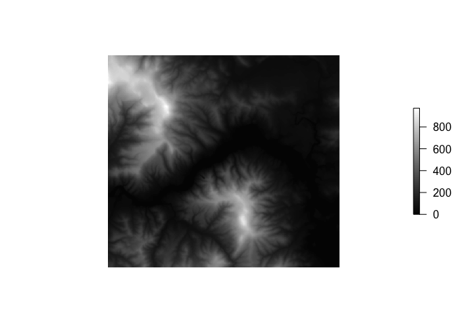

With rayshader, we can easily produce a realistic 3D visualisation of the same data.

library(rayshader)
library(magrittr)

# Generate a matrix from the tif data
elmat <- raster_to_matrix(tif)

elmat %>%
  sphere_shade(texture = "imhof2") %>%
  add_water(detect_water(elmat), color = "imhof2") %>%
  add_shadow(ray_shade(elmat), 0.5) %>%
  plot_3d(elmat, zscale = 10, shadow = FALSE, background = "#0f0e17",
          fov = 0, theta = 135, zoom = 1, phi = 45,
          solid = FALSE, windowsize = c(800, 500))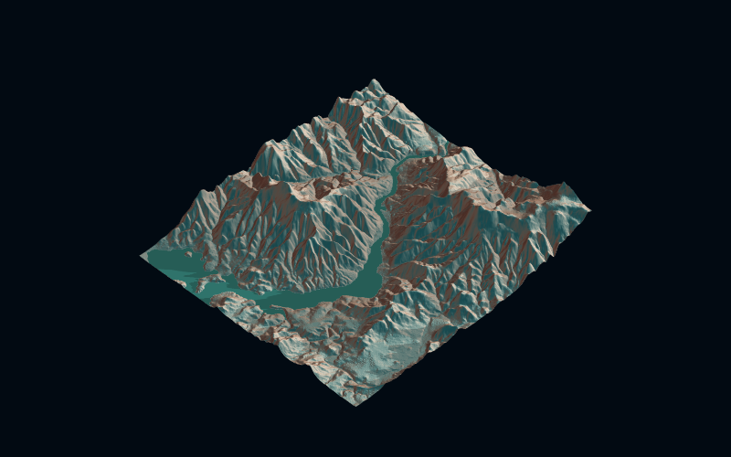

As this code shows, rayshader also provides a number of functions to enhance our visualisation by applying realistic shadows and shading to the topography, as well as adding water.

This 3D visualisation is much better representation of the underlying elevation data.

Recreating China’s Jade Dragon Snow Mountain with rayshader

The Jade Dragon Snow Mountain, 玉龙雪山, is a small mountain range in the north of Yunnan province in south-west China. It’s highest peak is around 5,600 metres above sea level.

Tyler Morgan-Wall, rayshader’s author, has provided an excellent guide on making 3D maps using satellite imagery. As my code closely follows Tyler’s example, I won’t post it all here - though it is available on GitHub.

One of the advantages of running this analysis in R is that the language has a huge ecosystem of spatial packages which can be used to prep and clean the data before we produce the visualisation. For instance, the elevation data from Derek Watkin’s SRTM tile downloader covered a much larger area the Jade Snow Mountain. To remedy this, I used the sf package to create a new simple feature collection out of two sets of lat long coordinates. The extent of these coordinates are then used to crop the elevation data.

library(sf)

point_1 <- c(y=100.05, x=27.25)
point_2 <- c(y=100.3, x=27.0)

extent_latlong <- st_sf(a = 1:2, geom = st_sfc(st_point(point_1), st_point(c(point_2))), crs = 4326)

e <- raster::extent(extent_latlong)

elevation_cropped <- raster::crop(elevation, e)

After importing and cleaning all the data, our plot_3d() call produced the following visualisation.

plot_3d(hillshade = rgb_contrast,
        heightmap = yu_long_matrix,
        zscale = 30, fov = 0, theta = 30, zoom = 0.5,
        phi = 20, solid = FALSE, windowsize = c(1200, 700),
        background = "#0f0e17", shadowcolor = "#0f0e17")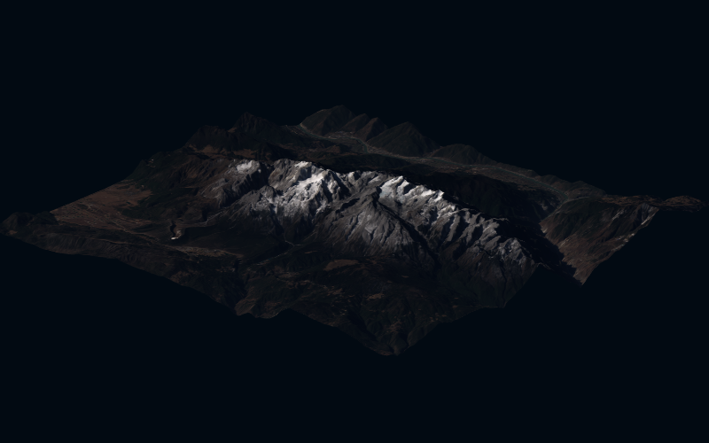

When we run the plot_3d() function locally, rayshader outputs to an rgl device that allows us to pan around our 3D visualisation. This got me thinking - how could I embed this interactive map into a web application?

Three.js and react-three-fiber

Three.js is the most widely used JavaScript library for displaying 3D graphics in a web browser. In three.js, three dimensional visualisations are constructed by arranging geometries, lights and cameras into a scene.

Three.js also uses a renderer to draw our scene to the user’s screen. This is an issue if you’re using a library like React, which relies on having exclusive control of the DOM.

Fortunately, the react-three-fiber library provides a React renderer for three.js. React-three-fiber also implements a declarative, component-based syntax that makes implementing three.js in a React application very simple.

From rayshader to React

Rayshader provides a function, save_obj(), to export our model as an .obj file. This function also exports the hillshade we’ve created (in our case the satellite imagery) as the model’s texture.

save_obj("outputs/yulongxueshan.obj", save_texture = TRUE)

.obj files tend to be too large to use in web browsers, so it’s necessary to convert them to a GLTF format. There are a few ways to achieve this, though I found the simplest way was to download open-source 3D software Blender. Blender has an option to import .obj files and then export as a .glb (one of the two file extensions associated with GLTF).

Another tool I found extremely useful was gltfjsx, which is also developed by the react-three-fiber team. This command-line tool turns GLTF assets into JSX components - effectively writing boilerplate code to import and manipulate our 3D object.

Creating our 3D components

The 3D model on this page is comprised of two function components - <Scene />, which houses the three.js scene and controls the state of the user inputs; and <RayshaderModel />, which load the model and applies some visual styles.

The <Scene /> components looks like this. Note that we’re importing the <OrbitControls /> component from the drei library. Drei provides a number of helper functions and abstractions for react-three-fiber that make it easy to add effects and interactions, such as shaders, controls or complex geometries.

import { useState, Suspense } from "react"
import { Canvas } from "react-three-fiber"
import { OrbitControls } from "drei"

const Scene = () => {
  const [orbit, setOrbit] = useState(false)
  const [overlay, toggleOverlay] = useState(true)

  return (
    <>
      <button onClick={() => toggleOverlay((prevState) => !prevState)}>
        Satellite overlay
      </button>
      <button onClick={() => setOrbit((prevState) => !prevState)}>
        Enable controls
      </button>
      <div style={{ height: 450, width: "100%" }}>
        <Canvas
          camera={{
            fov: 30,
            position: [0, 90, 150],
          }}
          shadowMap={true}
        >
          <ambientLight />
          <spotLight
            intensity={1}
            position={overlay ? [0, 100, 0] : [70, 20, 30]}
          />
          <pointLight position={[0, 20, 0]} color={"#FFFFFF"} intensity={0.4} />
          <Suspense fallback={null}>
            <RayshaderModel overlay={overlay} />
          </Suspense>
          {orbit && <OrbitControls />}
        </Canvas>
      </div>
    </>
  )
}

The code here is actually very simple. We have a couple of buttons to toggle the model’s texture (more on this later) and to enable orbit controls. We then draw the <Canvas />, where the 3D model lives as well as several lights for the scene.

One thing to note about react-three-fibre is that we can use components like <ambientLight /> and <pointLight /> without importing them. React-three-fiber abstracts this away.

In our <Canvas /> component, wrapped in <Suspense> tags, is our <RayshaderModel />. The code for this component is as follows.

import { useRef } from "react"
import { useLoader, useFrame } from "react-three-fiber"
import { GLTFLoader } from "three/examples/jsm/loaders/GLTFLoader"
import * as THREE from "three"

const RayshaderModel = ({ overlay }) => {
  const ref = useRef()
  const { nodes, materials } = useLoader(GLTFLoader, "/yuelongxueshan.glb")

  useFrame(() => {
    ref.current.rotation.y += 0.005
  })

  const overlayProps = {
    geometry: nodes.yulongxueshan.geometry,
    rotation: [Math.PI / 2, 0, 0],
    scale: [0.1, 0.1, 0.1],
    material: materials.ray_surface,
  }

  const materialProps = {
    geometry: nodes.yulongxueshan.geometry,
    rotation: [Math.PI / 2, 0, 0],
    scale: [0.1, 0.1, 0.1],
    receiveShadow: true,
    castShadow: true,
  }

  const props = overlay ? overlayProps : materialProps

  return (
    <group ref={ref}>
      <mesh {...props}>
        {!overlay && (
          <meshStandardMaterial
            color='#A87A65'
            roughness={0.7}
            metalness={0.7}
            side={THREE.DoubleSide}
          />
        )}
      </mesh>
    </group>
  )
}

useLoader.preload(GLTFLoader, "/yuelongxueshan.glb")

Let’s take a closer look at this component. One of the advantages of using gltfjsx is that it creates a nested graph of all the objects and materials inside our model. The boilerplate code returned to us by running gltfjsx provides these objects via the useLoader() hook.¹

Because we now have direct access to the geometry and textures within our model, we can swap or modify them. For instance, our <RayshaderModel /> component take a single prop - overlay. When overlay is true, we provide a set of props to the <mesh /> in our return statement that includes our rayshader surface.

When overlay is false, we instead provide an alternative sets of props to <mesh />, along with a child component, <meshStandardMaterial />. This child component provides an alternative texture to our geometry. This is only possible because gltfjsx has located our geometry and material within our .glb file and made them available to us directly.

We’re also using react-three-fiber’s useFrame() hook to animate our model. This hook allows us to apply calculations to our model on every frame calculation, which in three.js happens 60 times every second. Here, we use useFrame() to apply a very small increment to the y axis rotation of our model with every frame calculation.

Comparing our three.js and Rayshader visualisations

Our three.js visualisation lacks the sophisticated lighting effects that rayshader provides, and so our three.js model certainly looks less realistic than its rayshader counterpart.

However, because were were able to convert our .obj file from rayshader to a GLTF asset and integrate it into a React application, we’re able to provide a good looking and fast-loading 3D visualisation. Moreover, all the methods of managing user input and state that make developing applications in React so effective are now available to us.

Rayshader is a fantastic library, which has recently been updated to support adding 3D polygons passed as sf objects. I’m keen to explore how the library could potentially be used to create realistic representations of buildings and cities, particularly as the UK has made very high resolution elevation data available via the National Lidar Programme.

Likewise, I was amazed when reading the react-three-fiber docs how easy it is to integrate 3D models and effects into a React application. I’ll certainly be implementing these sorts of experiences into more projects in the future.