The Science Museum in London holds more than 325,000 objects in its exhibition halls and archives, including the world’s oldest surviving locomotive, the first jet engine and the Apollo 10 command module.
The Science Museum have made available information about each object in their collections via an api, which provides details of the object’s age, country of origin, materials and a text description.
In this article, we’re going to explore these text descriptions using
the tidytext package, and then build several machine learning models
using using the tidymodels package. These supervised learning models
will use the description of the object to identify whether it is an item
from the computing and data collection, or the space technology collection.
We’ll start by loading the tidyverse packages, which we’ll be using
throughout our analysis, and reading in the data. I’ve written a
separate script to query the api and export the descriptions as a csv file,
which is available on my
github.
The computing and space objects are in two separate csv files, so we’ll
read them in and then use bind_rows() to merge them.
library(tidyverse)

computing <- read_csv("data/computing-data-processing/objects.csv")
space <- read_csv("data/space/objects.csv")

objects <- bind_rows(list('computing' = computing, 'space' = space), .id = 'category') %>%
  distinct(description, .keep_all = TRUE)

objects %>% glimpse()
## Rows: 2,851
## Columns: 5
## $ category <chr> "computing", "computing", "computing", "computing", "computing", "computing", "computing", "computing", "computi…
## $ id <chr> "co408737", "co408742", "co408744", "co409177", "co409514", "co409516", "co409544", "co409546", "co409548", "co4…
## $ title <chr> "word processor", "Personal Computer by Memotech, 1980-1985, with man", "Heathkit model 88 personal computer kit…
## $ description <chr> "Personal Word Processor by Amstrad, model PCW 8256, with monitor, printer, documentation and software", "Person…
## $ url <chr> "https://collection.sciencemuseumgroup.org.uk/objects/co408737/word-processor", "https://collection.sciencemuseu…The description column in our data contains a text description of each object. These vary in length and format. Two somewhat typical examples are
below. We’ll analyse these descriptions using the tidytext package.
objects %>%
  filter(id == 'co408737') %>%
  pull(description)
## [1] "Personal Word Processor by Amstrad, model PCW 8256, with monitor, printer, documentation and software"objects %>%
filter(id == 'co433631') %>%
pull(description) ## [1] "Model of Apollo Command Service Module (CSM) and Lunar Excursion Module (LEM) in trans lunar configuration, scale 1:48."Text mining with tidytext
Tidytext
is a superb package for manipulating and analysing text data in R,
originally developed by Julia Silge and David Robinson. The first thing
we’ll do using tidytext is tokenise our descriptions - breaking each
description down into individual words. We’ll then remove from these
words any stop words - extremely common words that don’t add much to our
analysis, such as ‘the’, ‘and’ or ‘with’.
There are also a lot of numbers in our object descriptions. Sometimes these numbers have a particular significance - such as the year the object was produced - but often they’re an obscure product serial number. For our analysis, we’ll remove any numbers from our words.
library(tidytext)

object_descriptions <- objects %>%
  unnest_tokens('word', description, drop = FALSE) %>%
  anti_join(stop_words, by = 'word') %>%
  filter(!str_detect(word, "[0-9]"))

object_descriptions
## # A tibble: 34,635 x 6
## category id title description url word
## <chr> <chr> <chr> <chr> <chr> <chr>
## 1 computing co4087… word proc… Personal Word Processor by Amstrad, model PCW 8256, w… https://collection.sciencemuseumgroup.… personal
## 2 computing co4087… word proc… Personal Word Processor by Amstrad, model PCW 8256, w… https://collection.sciencemuseumgroup.… word
## 3 computing co4087… word proc… Personal Word Processor by Amstrad, model PCW 8256, w… https://collection.sciencemuseumgroup.… process…
## 4 computing co4087… word proc… Personal Word Processor by Amstrad, model PCW 8256, w… https://collection.sciencemuseumgroup.… amstrad
## 5 computing co4087… word proc… Personal Word Processor by Amstrad, model PCW 8256, w… https://collection.sciencemuseumgroup.… model
## 6 computing co4087… word proc… Personal Word Processor by Amstrad, model PCW 8256, w… https://collection.sciencemuseumgroup.… pcw
## 7 computing co4087… word proc… Personal Word Processor by Amstrad, model PCW 8256, w… https://collection.sciencemuseumgroup.… monitor
## 8 computing co4087… word proc… Personal Word Processor by Amstrad, model PCW 8256, w… https://collection.sciencemuseumgroup.… printer
## 9 computing co4087… word proc… Personal Word Processor by Amstrad, model PCW 8256, w… https://collection.sciencemuseumgroup.… documen…
## 10 computing co4087… word proc… Personal Word Processor by Amstrad, model PCW 8256, w… https://collection.sciencemuseumgroup.… software
## # … with 34,625 more rowsOnce we’ve done this we can explore the number of non-common words in our descriptions for each object. There are around 2,750 objects in our dataset, and approximately 1,000 of them have between 5 and 10 non-common words. A large number, around 850, have fewer than five non-common words.
object_descriptions %>%
  add_count(id) %>%
  distinct(category, id, n) %>%
  ggplot(aes(n)) +
  geom_histogram(binwidth = 5, boundary = 0, color = 'white') +
  geom_rug()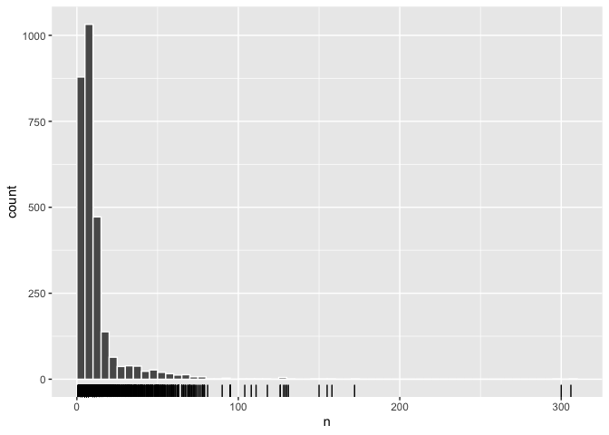
There are also some objects with very long descriptions. We might expect these to be the objects with greater historical significance, but this doesn’t really seem to be the case. While the Apollo 10 command module is among the longest descriptions, so are two descriptions for different versions of the same games console - the C64 and the C64 mini. Many of the other long descriptions are articles about space meals developed for British astronaut Tim Peak.
object_descriptions %>%
  count(title, description) %>%
  slice_max(n = 10, order_by = n)
## # A tibble: 10 x 3
## title description n
## <chr> <chr> <int>
## 1 The C64 Mini games console (video games) "Developed by Retro Games Ltd. the C64Mini is a retro games con… 306
## 2 The C64 games console (video games) "Developed by Retro Games Ltd. the C64 is a retro games console… 300
## 3 Space food, bacon sandwich made in collaboration with Heston… "This bacon sandwich was developed by celebrity chef, Heston Bl… 172
## 4 Pepys Series 'Astronaut' card game (card game) "‘Pepys’ is the brand name used by Castell Bros, a company foun… 158
## 5 Space food, Sausage sizzle made in collaboration with Heston… "This sausage sizzle dish was developed by celebrity chef, Hest… 155
## 6 Apollo 10 command module, call sign 'Charlie Brown' (manned … "The command module was the only part of the Apollo spacecraft … 150
## 7 Space food, Operation Raleigh (salmon) made in collaboration… "This Operation Raleigh (salmon) dish was developed by celebrit… 131
## 8 Space food, Stewed apples made in collaboration with Heston … "This stewed apples dish was developed by celebrity chef, Hesto… 130
## 9 Space food, chicken curry made in collaboration with Heston … "This chicken curry was developed by celebrity chef, Heston Blu… 129
## 10 Soyuz TMA-19M descent module, S.P. Korolev Rocket and Space… "The Russian made Soyuz TMA-19M spacecraft is the first flown, … 128What are the most common words in the descriptions?
One basic question we can ask of the data is what are the most common words in the computing and space collections. Looking at the visualisation below, we can see that within computing, ‘computer’, ‘game’ and ‘model’ are the most frequently used words. ‘Model’ is also a frequently used word in the space descriptions, though likely in a different context (e.g. a scale model of a rocket, etc), along with ‘rocket’, ‘scale’, ‘satellite’ and ‘space.‘
object_descriptions %>%
  count(category, word) %>%
  group_by(category) %>%
  slice_max(n = 20, order_by = n) %>%
  mutate(word = reorder_within(word, n, category)) %>%
  ggplot(aes(n, word)) +
  geom_col() +
  facet_wrap(~category, scales = 'free') +
  scale_y_reordered()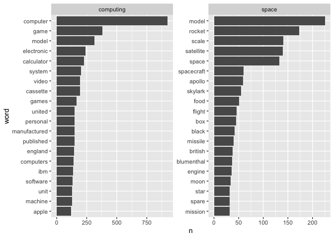
One limitation of merely counting words is that there are some terms which are likely to be common in each category, such as ‘model’. So rather than merely counting words, we can also estimate the how likely different words are to be found in each category using log odds.
We can calculate log odds using the bind_log_odds() function from the tidylo package.1 Looking at the graph below, we can see that words such as ‘calculator’,
‘video’, ‘cassette’ are much more likely to be found in the computing
descriptions. We can also see the presence of a number of brand names
that appear in the computing descriptions - ‘Apple’, ‘Nintendo’
and ‘Commodore’.
library(tidylo)

objects_log_odds <- object_descriptions %>%
  count(category, word) %>%
  bind_log_odds(category, word, n) %>%
  arrange(desc(log_odds_weighted))

objects_log_odds %>%
  group_by(category) %>%
  slice_max(log_odds_weighted, n = 20)  %>%
  mutate(word = fct_reorder(word, log_odds_weighted)) %>%
  ggplot() +
  geom_col(aes(log_odds_weighted, word, fill = category), show.legend = FALSE) +
  facet_wrap(~category, scales = "free")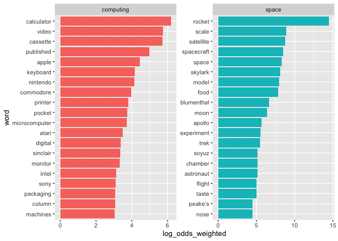
How are the words connected?
We may also be interested in which words often appear together within an
object’s description. We can estimate this for each group with the
pairwise_count() function from the widyr package. This code will
return a dataset of the number of times every word in our data
appears with every other word, calculated separately within each
category.
library(widyr)

word_pairs <- object_descriptions %>%
  group_by(category) %>%
  nest() %>%
  mutate(pairs = map(data, pairwise_count, word, id, sort = TRUE, upper = FALSE)) %>%
  select(-data) %>%
  unnest(pairs) %>%
  ungroup()

word_pairs
## # A tibble: 249,653 x 4
## category item1 item2 n
## <chr> <chr> <chr> <dbl>
## 1 computing game video 168
## 2 computing electronic calculator 144
## 3 computing cassette game 131
## 4 computing model computer 130
## 5 computing game published 129
## 6 computing video published 127
## 7 computing cassette published 123
## 8 computing cassette video 116
## 9 computing personal computer 103
## 10 computing england published 95
## # … with 249,643 more rowsWe can then visualise the connections between these words as network
graphs, using the ggraph package. Looking at the network graphs, we
can see that the word ‘computer’ connects many words within the computing collection, but
that there are also strong links between terms like ‘game’, ‘video’ and
‘cassette’.
library(ggraph)
library(igraph)

set.seed(42)

word_pairs %>%
  filter(category == 'computing', n > 30) %>%
  select(-category) %>%
  graph_from_data_frame() %>%
  ggraph(layout = 'fr') +
  geom_edge_link(aes(edge_alpha = n, edge_width = n), edge_colour = "cyan4") +
  geom_node_point() +
  geom_node_text(aes(label = name), vjust = 1, hjust = 1) +
  theme_void()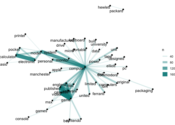
Our space network is somewhat sparser, but we can see that the strongest link is between ‘scale’ and ‘model’. We can also see links between ‘rocket’ and ‘engine’, and ‘motor’ and ‘chamber’.
set.seed(42)

word_pairs %>%
  filter(category == 'space', n > 15) %>%
  select(-category) %>%
  graph_from_data_frame() %>%
  ggraph(layout = 'fr') +
  geom_edge_link(aes(edge_alpha = n, edge_width = n), edge_colour = "hotpink") +
  geom_node_point() +
  geom_node_text(aes(label = name), vjust = 1, hjust = 1) +
  theme_void()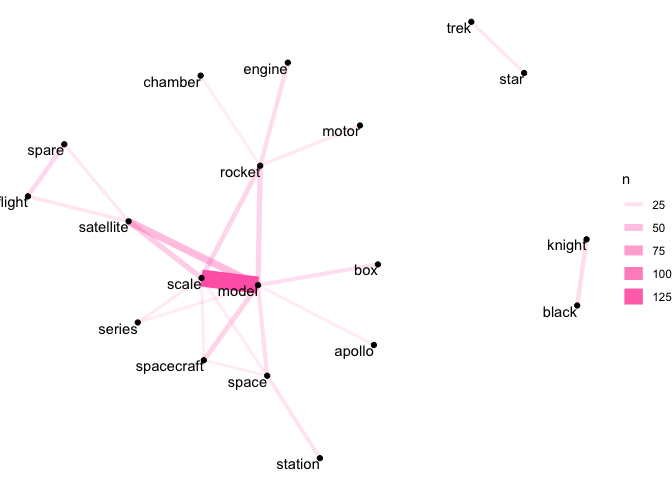
As with our earlier discussion of word counts, there are limits to what we can infer by looking at pairwise counts. ‘Scale’ and ‘model’ are common words in our space object descriptions, so it’s not too surprising that they’re frequently seen with other words.
We might instead be interested in the correlation between words, which
indicates how often these words appear together relative to how often
they appear separately. The widr package also provides a function for
this, pairwise_cor(), which uses the phi
coefficient.
keywords <- object_descriptions %>%
  group_by(category) %>%
  add_count(word) %>%
  ungroup() %>%
  filter(category == 'computing' & n > 20 | category == 'space' & n > 15)

word_cors <- keywords %>%
  group_by(category) %>%
  nest() %>%
  mutate(cor = map(data, pairwise_cor, word, id, sort = TRUE, upper = FALSE)) %>%
  select(-data) %>%
  unnest(cor) %>%
  ungroup()
We can then visualise these connections using the ggraph package, as
we did before.
Here, we can see in the computing category that the strongest correlations often relate to particular types of technology (‘circuit’ and ‘board’, ‘punched’ and ‘cards’, ‘word’ and ‘processing’) or brands (‘sony’ and ‘playstation’, ‘hewlett’ and ‘packard’, ‘intel’ and ‘microprocessor’).
set.seed(2021)

word_cors %>%
  filter(category == 'computing', correlation > 0.5) %>%
  select(-category) %>%
  graph_from_data_frame()  %>%
  ggraph(layout = 'fr') +
  geom_edge_link(aes(edge_alpha = correlation, edge_width = correlation), edge_colour = "cyan4") +
  geom_node_point() +
  geom_node_text(aes(label = name), vjust = 1, hjust = 1) +
  theme_void()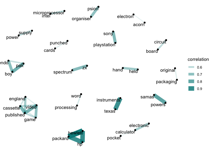
In the space collection, we can see a strong correlation between several objects related to space food. This is likely because, as we saw earlier, there were several objects related to this topic that reused a lot of the same words.
We can also see objects related to particular missions or programmes - e.g. ‘black’ and ‘knight’, related to the UK’s Black Knight missile research - or the popular culture space objects, evidenced by the correlation between ‘star’ and ‘trek’.
set.seed(2021)

word_cors %>%
  filter(category == 'space', correlation > 0.3) %>%
  select(-category) %>%
  graph_from_data_frame()  %>%
  ggraph(layout = 'fr') +
  geom_edge_link(aes(edge_alpha = correlation, edge_width = correlation), edge_colour = "hotpink") +
  geom_node_point() +
  geom_node_text(aes(label = name), vjust = 1, hjust = 1) +
  theme_void()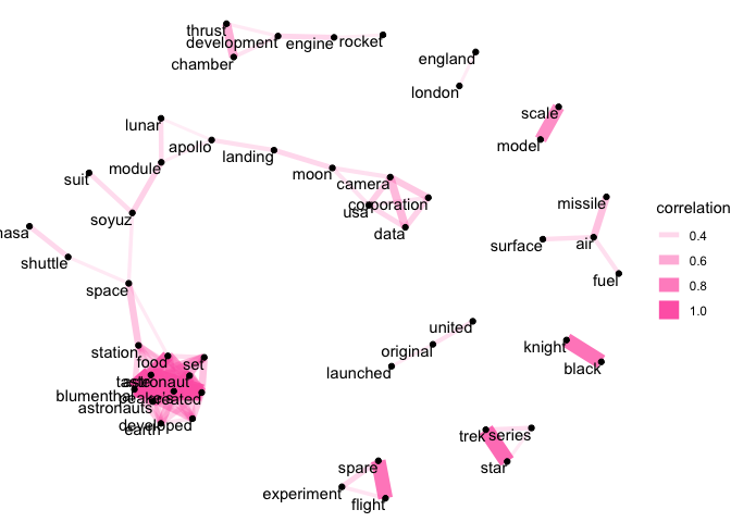
Machine learning with tidymodels
So far we’ve explored the descriptions of the computing and space
objects, getting a feel for the terms they use and the substance of the
descriptions. One thing we could do to extend this analysis is develop a
statistical model that predicts from looking at the object
descriptions whether it belongs in the computing or space collection.
We’ll fit a few different models using the tidymodels package.
Tidymodels is a collection of modeling packages that provides a
unified interface to many different statistical modeling packages. In
practice, this means we don’t need to remember the idiosyncrasies of a
particular model implementation, but simply follow some consistent steps
using tidymodels.
The first step in creating our model is to divide the data into separate datasets for training and testing.
library(tidymodels)

set.seed(42)

objects_split <- initial_split(objects, strata = category)
objects_training <- training(objects_split)
objects_testing <- testing(objects_split)
We want our training process to be as robust as possible, so we’ll also divide the c. 2,000 training data objects further into separate cross-validation ‘folds’. This process breaks our training data into ten roughly equally sized pieces, each known as a fold. The first fold will function like a test set in that we’ll use it to assess the performance of our model. The rest of the data will be used to train our model. We’ll repeat this dividing process ten times (creating ten slightly different models), and then average the performance across all the folds.
This gives us a good feel for whether our modeling approach is a good one before we touch the testing data. One important limitation with machine learning is that our training set is not a good arbiter of performance - a model built on the training data might overfit, producing impressive results which are not generalisable when we apply the model to the testing data. If we use cross-validation, this is less likely to occur because we’re creating ten different datasets to train and assess our approach.
set.seed(42)
objects_folds <- vfold_cv(objects_training, strata = category)
objects_folds
## # A tibble: 10 x 2
## splits id
## <list> <chr>
## 1 <split [1.9K/215]> Fold01
## 2 <split [1.9K/215]> Fold02
## 3 <split [1.9K/214]> Fold03
## 4 <split [1.9K/214]> Fold04
## 5 <split [1.9K/214]> Fold05
## 6 <split [1.9K/214]> Fold06
## 7 <split [1.9K/214]> Fold07
## 8 <split [1.9K/213]> Fold08
## 9 <split [1.9K/213]> Fold09
## 10 <split [1.9K/213]> Fold10Writing a model recipe
Now that we’ve separated our data, let’s think about the steps we need to take before we fit our model. As we’re interested in using the raw text descriptions to predict an object’s category, there are a number of processing steps we need to undertake.
In tidymodels, these processing
steps are part of a recipe, which specifies our model formula and all
the transformations we want to apply to our data before we fit a
model. Tidymodels comes with an extensive number of functions for
processing text data.
Our recipe involves first tokenizing the data and removing any stop
words. We also stem the words, which reduces the word to its base or
root form, using step_stem(). This means words like ‘astronauts’ will be
reduced to ‘astronaut’, or ‘computation’ to ‘compute’. This isn’t always
necessary, but given that many of our words are plurals or other
variations on more common words, it may help the model identify the
roots within each category of object. We’ll also use only the most common 500
words in our descriptions by specifying 500 to our step_tokenfilter().
We don’t use the actual words in our model. Instead, we take their term frequency inverse document frequency (tf-idf). The idea of the tf-idf is that it provides a numeric estimate of how important a word is in a collection of documents. A word that appears in every document, for instance, will have a tf-idf score of zero, and so is deemed unlikely to convey anything of particular significance in any one of the documents. We saw earlier that ‘model’ is a relatively common word across all of our object descriptions, so it will be assigned a lower tf-idf as it’s less likely to tell us much about whether the object is a space or computing object, compared with terms like computer or rocket.
Finally, we down-sample the category column so that we have a more equal proportion of space and computing objects in our data.
library(textrecipes)
library(themis)

additional_stop_words <- objects %>%
  unnest_tokens('word', description) %>%
  filter(str_detect(word, "[0-9]")) %>%
  pull(word)

model_recipe <- recipe(category ~ description, data = objects_training) %>%
  step_tokenize(description) %>%
  step_stopwords(description, custom_stopword_source = additional_stop_words) %>%
  step_stopwords(description) %>%
  step_stem(description) %>%
  step_tokenfilter(description, max_tokens = 500) %>%
  step_tfidf(description) %>%
  step_downsample(category)
We can now attach our model to a workflow. A workflow in
tidymodels bundles together our recipe and the model we’re going to
create. The advantage of this is that we can then swap one model for
another one, while keeping the recipe the same.
objects_workflow <- workflow() %>%
  add_recipe(model_recipe)
We’ll also want to create a null model, which we’ll compare to each of our statistical models. The null model will simply guess the modal class in our data on every prediction. In our case it will guess that every object is a computing object - as around three-quarters of our objects are computing objects, the null model will be right around three-quarters of the time. This is the threshold we’ll aim to beat with our statistical models.
null_classification <- null_model() %>%
  set_engine("parsnip") %>%
  set_mode("classification")

null_rs <- workflow() %>%
  add_recipe(model_recipe) %>%
  add_model(null_classification) %>%
  fit_resamples(objects_folds, metrics = metric_set(accuracy, sensitivity, specificity))

null_rs %>%
  collect_metrics()
## # A tibble: 3 x 6
## .metric .estimator mean n std_err .config
## <chr> <chr> <dbl> <int> <dbl> <fct>
## 1 accuracy binary 0.749 10 0.000507 Preprocessor1_Model1
## 2 sens binary 1 10 0 Preprocessor1_Model1
## 3 spec binary 0 10 0 Preprocessor1_Model1A naive Bayes model
Let’s start with a naive Bayes model, which are often good at making predictions from text data due to their ability to accommodate a large number of features. Naive Bayes models are commonly used to identify spam email, for instance.
Fitting a naive Bayes model with tidymodels is very simple, we simply
call the naive_Bayes() function and specify our mode (in our case
classification). Then we add our model to our model workflow.
library(discrim)

nb_spec <- naive_Bayes() %>%
  set_mode('classification') %>%
  set_engine('naivebayes')

objects_workflow <- objects_workflow %>%
  add_model(nb_spec)

objects_workflow
## ══ Workflow ═══════════════════════════════════════════════════════════════════════════════════════════════════════════════════════════
## Preprocessor: Recipe
## Model: naive_Bayes()
##
## ── Preprocessor ───────────────────────────────────────────────────────────────────────────────────────────────────────────────────────
## 7 Recipe Steps
##
## ● step_tokenize()
## ● step_stopwords()
## ● step_stopwords()
## ● step_stem()
## ● step_tokenfilter()
## ● step_tfidf()
## ● step_downsample()
##
## ── Model ──────────────────────────────────────────────────────────────────────────────────────────────────────────────────────────────
## Naive Bayes Model Specification (classification)
##
## Computational engine: naivebayesNow we can fit the model onto our cross-validated folds. We’ll use several metrics to evaluate performance - accuracy, which is the percentage of objects we identify correctly; sensitivity, which is the number of correct predictions for ‘computing’ divided by the number of computing objects; and specificity, which is the number of correct predictions for ‘space’ objects divided by the actual number of space objects.
Our naive Bayes model performs just as badly as our null model. Like our null model, it seems to optimise by simply predicting that everything is a computing object. It therefore has a sensitivity of 1, because it correctly identifies all the computing objects, but a specificity of rate of 0, because it never predicts that any object belongs in the space collection.
nb_model <- fit_resamples(
  objects_workflow,
  objects_folds,
  metrics = metric_set(accuracy, sensitivity, specificity)
)

collect_metrics(nb_model)
## # A tibble: 3 x 6
## .metric .estimator mean n std_err .config
## <chr> <chr> <dbl> <int> <dbl> <fct>
## 1 accuracy binary 0.749 10 0.000507 Preprocessor1_Model1
## 2 sens binary 1 10 0 Preprocessor1_Model1
## 3 spec binary 0 10 0 Preprocessor1_Model1A Random Forest Model
Let’s try a random forest model, which can also accommodate a large number of variables. To do this, we simply create a new model specification and update our workflow.
rf_spec <- rand_forest(trees = 1000) %>%
  set_engine("randomForest") %>%
  set_mode("classification")

objects_workflow <- objects_workflow %>%
  update_recipe(model_recipe) %>%
  update_model(rf_spec)
We can then fit this model to our resamples and evaluate its
performance. Note that one of the disadvantages of a random forest model
with so many variables fitted over 10 folds is that it’s computationally
very expensive. For this reason, we use
doParallel::registerDoParallel() to run the model fitting on several
cores at the same time.
The random forest model performs excellently - correctly identifying 95% of our objects, and achieving a sensitivity and specificity rate of 97% and 90% respectively.
doParallel::registerDoParallel()

set.seed(2021)

rf_model <- fit_resamples(
  objects_workflow,
  objects_folds,
  metrics = metric_set(accuracy, sensitivity, specificity)
)

rf_model %>%
  collect_metrics()
## # A tibble: 3 x 6
## .metric .estimator mean n std_err .config
## <chr> <chr> <dbl> <int> <dbl> <fct>
## 1 accuracy binary 0.953 10 0.00455 Preprocessor1_Model1
## 2 sens binary 0.971 10 0.00409 Preprocessor1_Model1
## 3 spec binary 0.898 10 0.0150 Preprocessor1_Model1A Support-Vector Machine Model
Although the random forest results were very promising, we might just want to compare them to another model. This time we’ll use a Support-Vector Machine model (SVM).
SVMs are mathematically very complicated, but can be reasonably well understood with a simple heuristic. An SVM attempts to identify a boundary (known as a hyperplane) which separates data into fairly homogeneous groups. In a two dimensional space, this can be understood as a straight line drawn over a set of x and y coordinates that divides a number of points into two camps, with each camp representing something meaningful in the data.
In practice, SVMs can partition data over many different dimensions and can also be tweaked to adjust their operations when a clean split between groups in the data isn’t possible (something we’ll get to later).
We’ll first create a spec, and then update our objects_workflow with
the new model.
svm_spec <- svm_rbf() %>%
  set_mode("classification") %>%
  set_engine("liquidSVM")

objects_workflow <- objects_workflow %>%
  update_model(svm_spec)
We can then fit this model to our resamples and evaluate its performance.
doParallel::registerDoParallel()

set.seed(2021)

svm_rs <- fit_resamples(
  objects_workflow,
  objects_folds,
  metrics = metric_set(accuracy, sensitivity, specificity),
)
Our SVM model performs almost as well as our random forest model in terms of accuracy and sensitivity, and actually performs better at correctly identifying our space objects.
svm_rs_metrics <- collect_metrics(svm_rs)

svm_rs_metrics
## # A tibble: 3 x 6
## .metric .estimator mean n std_err .config
## <chr> <chr> <dbl> <int> <dbl> <fct>
## 1 accuracy binary 0.927 10 0.00712 Preprocessor1_Model1
## 2 sens binary 0.929 10 0.00740 Preprocessor1_Model1
## 3 spec binary 0.918 10 0.0169 Preprocessor1_Model1Tuning our SVM Model
One way we could try and boost the SVM’s performance further is by tuning some of its parameters. In our SVM model, there are two parameters we might want to tune - cost and sigma.
The cost parameter is used to adjust a penalty that’s applied to the model when our hyperplane can’t neatly separate our data into meaningful camps. The greater the cost parameter, the harder the model will try to achieve total separation. While it may sound like a higher cost is always better, it’s important to recognise that optimising too much to our training data will possibly result in worse performance on our testing data as our model won’t generalise well.
The sigma parameter (often also referred to as the gamma) determines the influence that each observation may exert on where the hyperplane is placed.
We can easily identify the optimal values for these parameters using a tuning grid.
First, we’ll create a new SVM model spec where we’ll state that we want
to tune the cost and rbf_sigma parameters.
svm_spec_tuned <- svm_rbf(cost = tune(), rbf_sigma = tune()) %>%
  set_mode('classification') %>%
  set_engine('liquidSVM')

objects_workflow <- objects_workflow %>%
  update_model(svm_spec_tuned)
We’ll now generate a grid of these parameters. Tidymodels
provides functions to help us select sensible values for each. We’ll set
levels equal to five, so that we are given five cost values and five
sigma values. The grid combines each value, giving us 25 different
pairs of cost and sigma to try.
param_grid <- grid_regular(cost(), rbf_sigma(), levels = 5)We’ll now fit 25 different models (each with a different set of parameters) onto ten different training folds - in effect, we’re about to fit 250 models. Again, because of the computation involved, we’ll set up parallel processing.
doParallel::registerDoParallel()

set.seed(2021)

tune_rs <- tune_grid(
  objects_workflow,
  objects_folds,
  grid = param_grid,
  metrics = metric_set(accuracy, sensitivity, specificity),
  control = control_resamples(save_pred = TRUE)
)
We can then collect the performance metrics and identify which parameter set produced the best results. Our model with the lowest cost parameter and a sigma of one performed the best. Even this model, however, doesn’t quite achieve the performance seen in our earlier random forest model.
show_best(tune_rs, metric = "accuracy") ## # A tibble: 5 x 8
## cost rbf_sigma .metric .estimator mean n std_err .config
## <dbl> <dbl> <chr> <chr> <dbl> <int> <dbl> <fct>
## 1 0.000977 1 accuracy binary 0.919 10 0.00600 Preprocessor1_Model21
## 2 0.0131 1 accuracy binary 0.354 10 0.00956 Preprocessor1_Model22
## 3 0.177 1 accuracy binary 0.331 10 0.00855 Preprocessor1_Model23
## 4 2.38 1 accuracy binary 0.331 10 0.00855 Preprocessor1_Model24
## 5 32 1 accuracy binary 0.331 10 0.00855 Preprocessor1_Model25Finalising our model
We’ve now used three different types of model and identified that our random forest model appears to be the best performing one. Let’s finalise our model and apply it to our testing data. We’ll first amend our workflow to using the random forest specification we defined earlier.
objects_workflow <- objects_workflow %>%
  update_model(rf_spec)
We now use the last_fit() function to construct the model using our
full training set, and then fit the model to our testing set.
final_res <- objects_workflow %>%
  last_fit(objects_split, metrics = metric_set(accuracy, sensitivity, specificity))
The model performs extremely well on the testing set, achieving an accuracy of 96%. It correctly identifies 97% of the computing objects, and 91% of the space objects.
final_res_metrics <- collect_metrics(final_res)
final_res_metrics
## # A tibble: 3 x 4
## .metric .estimator .estimate .config
## <chr> <chr> <dbl> <fct>
## 1 accuracy binary 0.961 Preprocessor1_Model1
## 2 sens binary 0.976 Preprocessor1_Model1
## 3 spec binary 0.916 Preprocessor1_Model1Now that we have our final model fit, we can also examine the importance
of different variables in our model. We do this using the vip package,
which provides functions for calculating the importance of variables
across many types of machine learning algorithms.
Looking at the figure below, we can see some of the most important variables to our model - the tf-idf scores of the words ‘compute’, ‘rocket’, ‘satellite’, ‘scale’ and ‘game’. We might infer from this that descriptions which feature these words or related ones are relatively easy for our model to classify correctly.
library(vip)

final_res %>%
  pluck('.workflow', 1) %>%
  pull_workflow_fit() %>%
  vip(num_features = 20)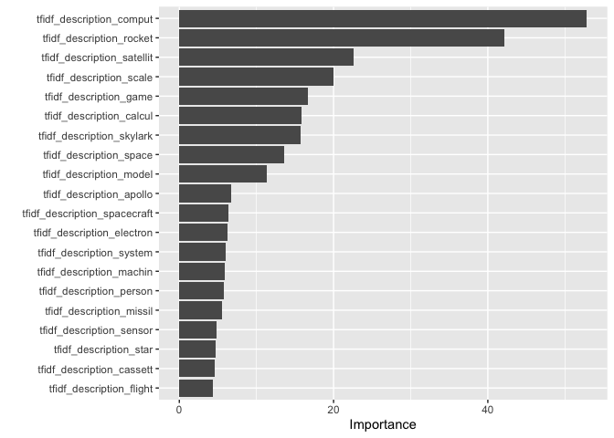
We can also take a closer look at the incorrect predictions. There’s nothing in these that seems particularly telling, other than some of these contain terms that are likely to be found in both the space and computer collections, such as the description of ‘Flown NASA Shuttle Main Guidance computer, IBM 1980’s’. Perhaps even a human would struggle to place this in the correct collection.
incorrect_preds <- collect_predictions(final_res) %>%
  filter(.pred_class != category) %>%
  pull(.row)

objects[incorrect_preds, ] %>%
  pull(description)
    ##  [1] "Optical Scanning Device Model OpScan 12/17 made by Optical Scanning Corporation, Pennsylvania, USA.  c1973."
    ##  [2] "2 paper folders formerly belonging to Charles Babbage containing cut-outs of gearwheels, cams etc. in thin card. One folder marked \"Models\" the other marked \"Models of rejected contrivances\""
    ##  [3] "Stereotype duplicate from a matrix produced on the Scheutz difference engine. Remarks: to be used, when required, as block for printing purposes"
    ##  [4] "Two double-sided flexible disc drives by Tandon model TM100"
    ##  [5] "Tensile strength testing machine for small gauge wires, made by GEC c1960. Used for testing semiconductor quality connection wires in late 1960's to early 1970's"
    ##  [6] "AES model Alpha Keyboard"
    ##  [7] "Keyboard, model no.LK201AE, s/n B030804823"
    ##  [8] "Monitor, model VR201, s/n TA27971"
    ##  [9] "Drum Kit prototype for Harmonix Rock Band, 2007."
    ## [10] "Capacitive fingerprint reader and associated software -  USB technical evaluation kit including individual sensors by AuthenTec,  United States, 1998-2008"
    ## [11] "Mechanical comptometer by Felt & Tarrant, Chicago, and used by the Manchester Guardian and Evening News."
    ## [12] "Apple iPad 2, Black, 16GB, Wi-Fi, Model A1395, designed by Apple in California, assembled in China, 2011-2012"
    ## [13] "Wiring and components from model CPT8100, by CPT corp., c.1980-1985."
    ## [14] "UK3 telecommand receiver"
    ## [15] "UK4 telemetry transmitter"
    ## [16] "UK4 telemetry package"
    ## [17] "Encoder modules (2 unpotted, 2 potted)"
    ## [18] "Power storage control unit"
    ## [19] "Skynet II hydrazine propulsion system"
    ## [20] "Channel electron multiplier"
    ## [21] "Whirlpool water gun-fire extinguisher"
    ## [22] "Ariel 3 type battery pack"
    ## [23] "Twelve STSA2 thermal shield material discs, 1993."
    ## [24] "Glass tankard with inscription \"Mars revisited 1976-1996 Lockheed Martin\", made 1996."
    ## [25] "Flown NASA Shuttle Main Guidance computer, IBM 1980's"
    ## [26] "Dr Who fighter spaceship; military air transport service 3112."
    ## [27] "Box for Cyberman alien scalemodel from television series Dr Who made by Sevans, Trowbridge, c.1987"
    ## [28] "Circuit board from IBM System 360 computer."
In this analysis we’ve performed some fairly advanced techniques for analysing and modelling text data, including fitting three machine learning models to identify which collection different objects from the Science Museum belong to.
The two packages we used most to do this,
tidyText and tidymodels, provide intuitive and easy-to-understand
interfaces to these complicated areas of data analytics and machine learning.
There are some great resources available on these packages, I would
recommend looking at Text Mining with
R, Supervised Machine Learning for
Text Analysis in R and Julia Silge’s fantastic
YouTube
channel to learn more.